Association Rule Mining in R

The dataset: A data set recording the disabilities of 21574 elderly people in the United States of America was collected as part of the National Long Term Care Survey (NLTCS). Each person’s disability in sixteen tasks of daily living were recorded. Six of the tasks are categorized as activities of daily living (ADLs) and ten are categorized as instrumental activities of daily living (IADLs).

Variable with Description:
Y1 eating
Y2 getting in/out of bed
Y3 getting around inside
Y4 dressing
Y5 bathing
Y6 getting to the bathroom or using toilet
Y7 doing heavy house work
Y8 doing light house work
Y9 doing laundry
Y10 cooking
Y11 grocery shopping
Y12 getting about outside
Y13 traveling
Y14 managing money
Y15 taking medicine
Y16 telephoning

Let us analyse the NLTCS dataset with the intention of finding the insightful association rules. Firstly, let us load the required R libraries and the dataset:

library(arules)
library(arulesViz)

dat <- read.table("http://mathsci.ucd.ie/~brendan/data/Old/nltcs.txt",header=TRUE)
head(dat)

##   Y16 Y15 Y14 Y13 Y12 Y11 Y10 Y9 Y8 Y7 Y6 Y5 Y4 Y3 Y2 Y1 COUNT
## 1   0   0   0   0   0   0   0  0  0  0  0  0  0  0  0  0  3853
## 2   0   0   0   0   0   0   0  0  0  0  0  0  0  0  0  1     4
## 3   0   0   0   0   0   0   0  0  0  0  0  0  0  0  1  0     9
## 4   0   0   0   0   0   0   0  0  0  0  0  0  0  1  0  0    19
## 5   0   0   0   0   0   0   0  0  0  0  0  0  0  1  0  1     1
## 6   0   0   0   0   0   0   0  0  0  0  0  0  0  1  1  0     8
##        PERCENT
## 1 17.859460462
## 2  0.018540836
## 3  0.041716881
## 4  0.088068972
## 5  0.004635209
## 6  0.037081672

In this analysis, we will be utilizing support, confidence and lift to guide through and mine the rules. We will make use of Fréchet bounds and apriori algorithm to calculate the support, confidence and lift. Let us approach the rule mining with two perspectives: in the first one, we will keep on changing thresholds for support and confidence and arrive at reasonable thresholds. Secondly, we will mine rules with different number of elements in the antecedent.

We will generate the transactions out of our dataset.

# Count how many patterns occur in the data and call it M.
M <- nrow(dat)
# Make a vector of numbers from 1 to M.
indices <- 1:M
# Extract the count for how often each pattern happens.
counts <- dat$COUNT
# Construct a vector where the row number of each pattern
# records the number of times that the pattern arises
# in the data. The rep() command is used for this.
rowindices <- rep(indices,counts)
# Now, let’s create the matrix nltcsmat.
nltcsmat <- dat[rowindices,]
# Let’s drop the last two columns because they’re not needed
nltcsmat <- nltcsmat[,-(17:18)]
# Let’s reorder the columns, so that they give disabilities
# from 1 to 16 instead of 16 to 1.
nltcsmat <- nltcsmat[,16:1]
# Let’s coerce the data.frame into a matrix.
nltcsmat <- as.matrix(nltcsmat)
# Transcactions
nltcs <- as(nltcsmat,"transactions")

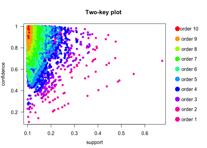
With initial values of support and confidence being 0.1, a priori algorithm mined 21483 rules. To understand the number of rules with variations in support and confidence, let us visually represent the rules with the help of support vs. confidence two-key plot. From this plot, it is evident that a large number of rules are in lower values of support, with interesting rules lying in higher values of support and confidence.

sup = 0.1
conf = 0.1

fit<-apriori(nltcs,parameter=list(support=sup, confidence=conf))

fit<-sort(fit,by="support")
plot(fit, method = "two-key plot")

Let us increase the support and confidence thresholds to see if we can find interesting rules.

conf = 0.5

fit<-apriori(nltcs,parameter=list(support=sup, confidence=conf))

fit<-sort(fit,by="support")

Increasing the confidence threshold to 0.5 gave 21215 rules, suggesting that large number of observations have high confidence. So, let us increase the support threshold and have a look at the number of rules mined, since only the most statistically evident and handful number of rules can be interpreted.

sup = 0.4
conf = 0.5

fit<-apriori(nltcs,parameter=list(support=sup, confidence=conf))

fit<-sort(fit,by="support")
inspect(fit)

##     lhs      rhs   support   confidence lift     count
## [1] {}    => {Y7}  0.6756744 0.6756744  1.000000 14577
## [2] {}    => {Y12} 0.5546028 0.5546028  1.000000 11965
## [3] {Y12} => {Y7}  0.4745064 0.8555788  1.266259 10237
## [4] {Y7}  => {Y12} 0.4745064 0.7022707  1.266259 10237
## [5] {Y11} => {Y7}  0.4453045 0.9169610  1.357105  9607
## [6] {Y7}  => {Y11} 0.4453045 0.6590519  1.357105  9607
## [7] {Y13} => {Y7}  0.4355706 0.8833427  1.307350  9397
## [8] {Y7}  => {Y13} 0.4355706 0.6446457  1.307350  9397

With support and confidence thresholds set at 0.4 and 0.5 respectively, we mined 8 rules. The redundant rules are removed from the list so that we analyse only the significant rules. Here, the tabulation shows the 8 rules mined and the corresponding quality measures. The -Inf and Nan for Standardized Lift for rules [7] and [8] indicate that lower bounds, upper bounds and lifts are all 1.0.

When sorted by support, the first two rules have empty antecedents (lhs), suggesting that these patients have condition such that they only have disability in the consequent. Let us have a look at the first rule: 14577 people in this dataset have only disability, Y7 (doing heavy house work). This make sense, since disabled people are more likely to manage their daily tasks, such as eating, taking medicine, telephoning pretty well but they are not that comfortable doing heavy housework. In this observation, the support of 0.67 suggests that the probability of none in lhs and disability Y7 (doing heavy house work) in rhs co-occurring together is 67%. Also, the confidence of 0.67 indicates that the probability that disability Y7 (doing heavy house work) is observed, given that no other disability is witnessed is 67%. Since this observation has lift equal to 1, it signifies that antecedent and consequent are independent of each other.

Now that we have seen an example of empty antecedent, let us examine the antecedents with increased lengths with same support and confidence thresholds. With lhs and rhs having 1 elements, we have 6 rules: {Y12} => {Y7}, {Y7} => {Y12}, {Y11} => {Y7}, {Y7} => {Y11}, {Y13} => {Y7} and {Y7} => {Y13}. The most prominent one {Y12} => {Y7} signifies that probability of Y12 (getting about outside) and Y7 (doing heavy house work) co-occurring together and given a person has Y7 (doing heavy house work), it is likely that Y12 (getting about outside) disability is seen. This is understandable since people who have difficulty doing heavy work are likely to face difficulty getting about outside. This rule has lift of 1.26 indicating that the degree to which those two occurrences are dependent on one another. Also, these 6 rules come in pairs of reversed lhs and rhs, with Y7 (doing heavy house work) being common among all.

If we observe rules with 2 antecedents and stretch back support and confidence to 0.3 and 0.5 respectively, we observe several interesting rules based on confidence measure. The probability of disability Y7 (doing heavy house work), given disabilities Y9 (doing laundry) and Y11 (grocery shopping) is 0.98. Also, chance of disability in Y12 (getting about outside), given disability in Y3 (getting around inside) and Y7 (doing heavy house work) is 93%.

Along with the individual probabilities PA and PB, we also calculated the upper and lower bounds for the lift governed by Fréchet bounds. With the help of these upper and lower bounds, tighter ranges of support and confidence, standardized lift is found to ensure we do not miss any interesting rules. In our 8 rules we mined, standardized lift is below 1.

With support threshold at 0.3 and confidence threshold at 0.5, we mined 58 rules, with redundant rules removed. We can visualize these rules with help of arulesViz package:

sup = 0.3
conf = 0.5

fit<-apriori(nltcs,parameter=list(support=sup, confidence=conf))

fit<-sort(fit,by="support")
plot(fit, method = "two-key plot")

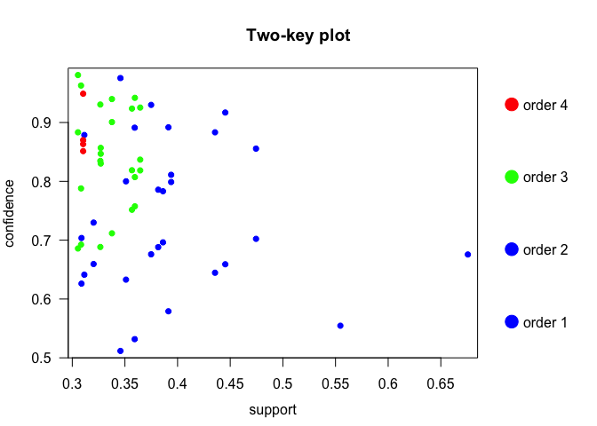
It is evident from the Two-key plot that we have very few rules with support greater than 0.5. Most of the rules are equally distributed with confidence between 0.5 and 1.0.

To conclude, association rules help us to mine interesting rules from any convoluted dataset. With proper utilization of Fréchet bounds, quality measures such as support, confidence and lift, we were able to understand our dataset and mine rules. This can be used for further statistics.

We got many insights some of which are summarized here:

1. Disabled people are more likely to manage their daily tasks, such as eating, taking medicine, telephoning pretty well but they are not that comfortable doing heavy housework.
2. It is evident that doing heavy housework has high individual associations with grocery shopping, getting about outside and traveling, which indicates that if the later 3 are seen, the person is likely to face difficulty in doing heavy housework.
3. If a person is facing issues in getting around inside and doing heavy house work, there is 93% chance that he/she will face issues in getting about outside.